MoCoSFL: ENABLING CROSS-CLIENT COLLABORATIVE SELF-SUPERVISED LEARNING

Contents

• 1. Introduction
• 2. Foundation Algorithms
  • 2.1 MoCo - Momentum Contrast
  • 2.2 SFL - Split Federated Learning
• 3. Deep Dive into the Paper
  • 3.1 Problem
  • 3.2 MoCoSFL
  • 3.3 TAResSFL - Target-Aware ResSFL
• 4. Experiments
• 5. References

1. Introduction

In this paper, we will explore the MoCoSFL algorithm, a prominent paper published in the top 5% at ICLR 2023 [3].

Before diving into MoCoSFL (Momentum Contrastive Self-Supervised Learning), we will first review MoCo (Momentum Contrast) and SFL (Split Federated Learning) to gain a comprehensive understanding of MoCoSFL.

2. Foundation Algorithms

2.1 MoCo - Momentum Contrast

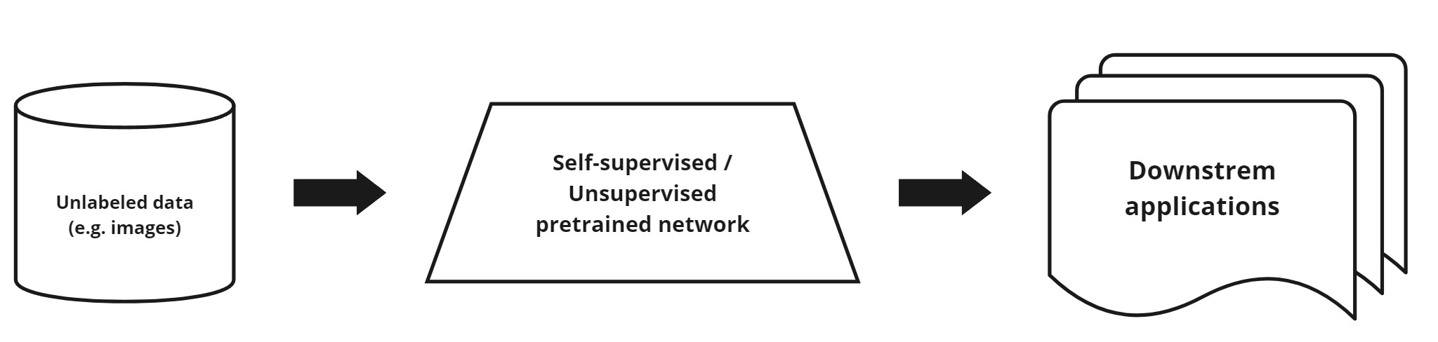Figure 1. Pipeline of Unsupervised Pretraining and Downstream Applications.

MoCo (Momentum Contrast) is a self-supervised learning method used to learn data representations without labels [1]. In MoCo, the goal is to build an encoder that can generate stable and effective representations from raw data such as images.

Reference Video: MoCo (+ v2) - Unsupervised learning in computer vision

MoCo operates on the idea of creating a dynamic dictionary of representations that are updated over time. The encoder is divided into two parts: a main encoder and a momentum encoder. The momentum encoder is updated slowly from the main encoder, helping to maintain consistency of representations over time. By comparing the representations of similar (positive pairs) and dissimilar (negative pairs) data, MoCo can learn meaningful features of the data without requiring labels.

This method has achieved good results in representation learning tasks, especially in learning useful representations for supervised tasks such as image classification and object recognition.

I have noted the video above in the way I understand here.

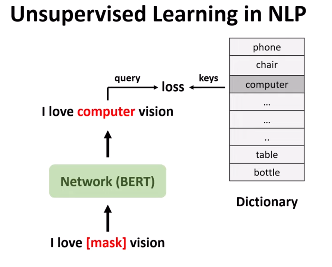Figure 2. Unsupervised learning in NLP.

In the context of unsupervised learning in NLP as illustrated in the figure, we consider a pre-trained model like BERT. We provide it with an input sequence such as “I love [mask token] vision” and the model's task is to predict the missing word, i.e., [mask token], with the highest probability from the dictionary, and then provide the replacement word. To achieve this, we have a dictionary containing all possible replacements for [mask token], and the model's job is to find the correct word. In this case, the machine applies a loss function between the missing word or [mask token] and the corresponding word in the dictionary, resulting in the sequence “I love computer vision”.

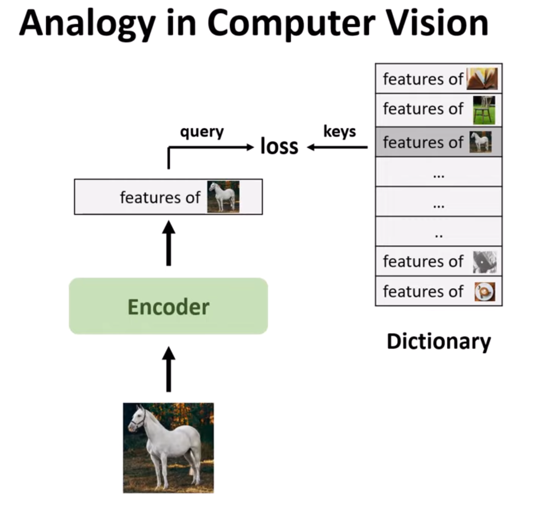Figure 3. Unsupervised learning in CV.

Similarly, in computer vision, we have an input image and pass it through an encoder to extract high-level features of that image. The dictionary in this case contains features of all possible images. This differs from NLP dictionaries due to the continuous and high-dimensional nature of image signals, compared to discrete signal spaces (like words or subword units) in NLP. The task is to find the exact feature from this dictionary and apply a loss function between the Query and Key. Since only features are extracted from images, contrastive learning is used to solve this problem.

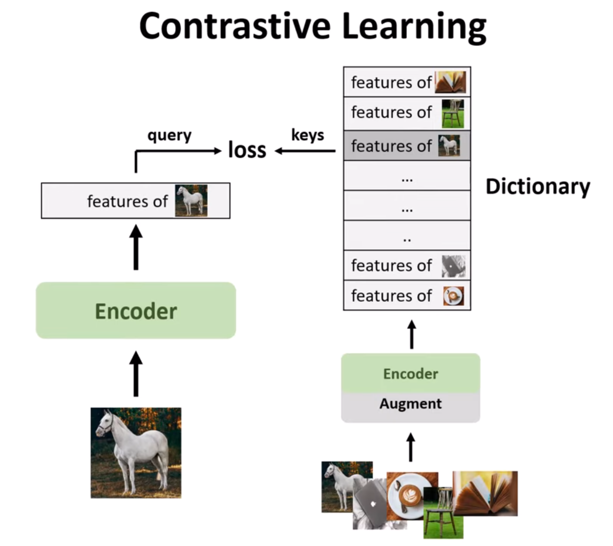Figure 4. Contrastive learning.

In contrastive learning, a batch of images is processed, and only the features from one of them are used as the query. For the batch of images, various data augmentation techniques such as color changes, reflections, etc., are applied to create augmented versions. These are then used to build the dictionary with features being augmented versions of the original image. Since we know which features come from augmented versions of the query image, we apply a loss function between the feature of the query image and its augmented features.

Figure 5. Visualization of data augmentation.

Adding data augmentation to the original image results in multiple augmented images. Features extracted from these images are compared to ensure they are as similar as possible, which is beneficial as different augmentations are applied across different epochs, making the model more robust to data augmentation and better at learning from these images.

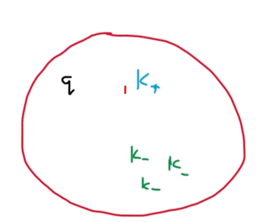Figure 6. Solution space.

Next, we consider the loss function. In contrastive learning, we have a solution space where both the query and all its keys reside. The task is to apply a loss function to pull the query and positive key closer together in this space while pushing all negative keys from different images away. This results in a better decision boundary for classification and other tasks. Here is the formula for the loss function:

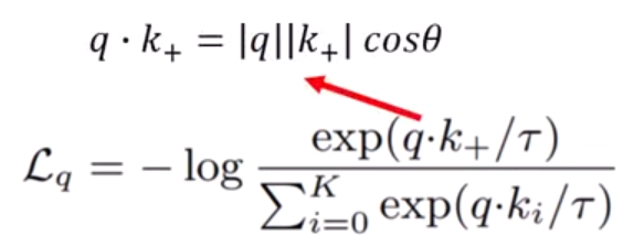Figure 8. Loss function of contrastive learning.

The loss function is embedded within a negative log function. Since the log function always increases, to decrease the negative log, we need to maximize what is inside it. To maximize, we need to maximize the numerator and minimize the denominator. The numerator contains the dot product of the positive key and query key, which is the norm of the vector and cosine of the angle between them. We aim to maximize this term as it signifies that the features are closer together. Cosine values range between 1 and -1, and to maximize it, the angle between the query and positive key should be zero, meaning they are aligned. Conversely, we minimize the denominator.

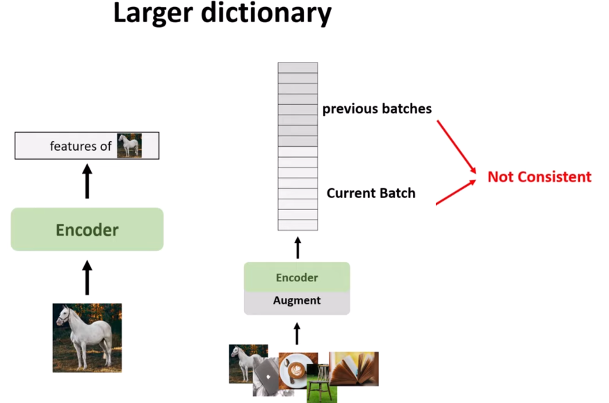Figure 9. Larger dictionary.

A larger dictionary increases the number of negative keys (and hard negative keys), requiring the model to push more negative keys away from the query, thus helping the model to learn better. However, there is a GPU memory limit, so we cannot increase the batch size in the usual way. Instead, a queue can be used to create a larger batch size for learning. The challenge is that each stack or batch is extracted from different encoders, making the features inconsistent, which is where momentum contrast comes in.

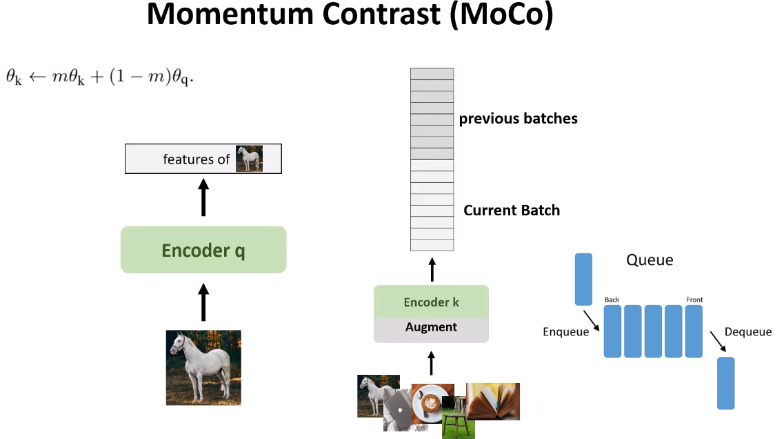Figure 10. Momentum contrast.

MoCo makes the dictionary independent of batch size by using two different encoders: one for the query and one for the key. It applies momentum updates to the key encoder to gradually update and make all stacks almost consistent. A value close to 1, such as 0.9 or 0.99, is used to keep the current weight of the key encoder as stable as possible. Features from the previous and current batches may differ slightly, but the first and last stacks will differ significantly. This is why a stack size of around 50 is often considered optimal.

2.2 SFL - Split-Federated Learning

For a detailed overview of Federated Learning, please refer to my article on Federated Learning.

Figure 11. Federated Learning Process.

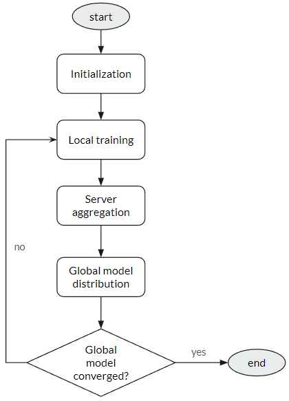To recap federated learning: There are 5 steps in the federated learning process:

1. Initialization: The central server initializes a shared model, distributed to all participating devices.
2. Local Training: Each device trains the model on its local data, using stochastic gradient descent or other optimization algorithms.
3. Model Aggregation: Devices send updated model parameters back to the central server, which aggregates them to create an improved global model.
4. Model Distribution: The central server distributes the updated global model back to the devices.
5. Repeat: The above steps are repeated until the model converges to an optimal state.

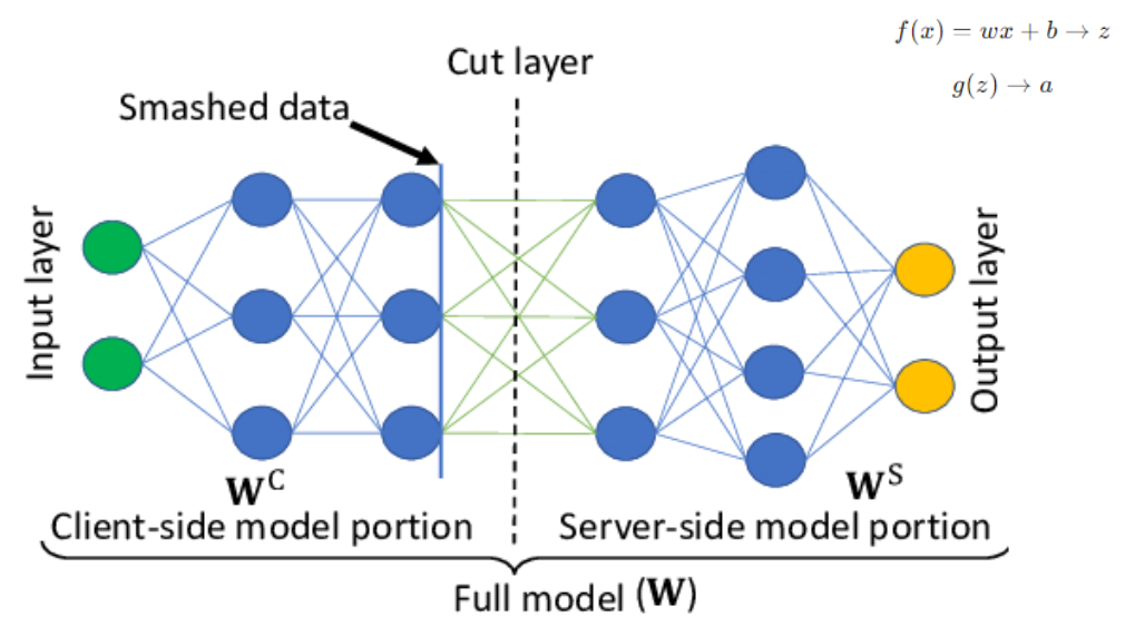Figure 12. Split Learning.

In split learning, the model is divided into 2 parts: one part is the client-side (frontend) and the other part is the server-side (backend). According to forward propagation in deep learning, after inputting data into a layer, that layer computes a vector z with weights and biases, then applies an activation function and returns a vector (which we can call a latent vector). The data at the cut layer is called smashed data, which is the latent vector sent to the server to continue the propagation process.

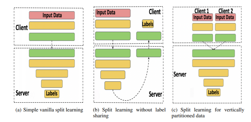Figure 12. There are 3 types in Split Learning.

(a) Simple Vanilla Split Learning

• Description: In this configuration, the neural network is split between the client and server. The client processes data through the initial layers and sends intermediate output to the server to complete the forward pass, perform backpropagation, and update weights.
• Process:
  1. Client Side: The client processes input data through a few initial layers of the neural network.
  2. Server Side: The server receives output from the client’s layers, processes it through the remaining layers, and calculates the loss using labels.
  3. Backpropagation: The server calculates gradients and sends them back to the client to update weights in the client-side layers.

(b) Split Learning without Label Sharing

• Description: This variant is designed to protect privacy by ensuring that the server does not have access to labels.
• Process:
  1. Client Side: The client processes input data through a few initial layers and keeps the labels.
  2. Server Side: The server processes output from the client’s layers through its own layers and sends back final results (without accessing labels).
  3. Client Side: The client calculates loss using labels and performs backpropagation through its layers. The client then sends the required gradients to the server to complete the backpropagation process.

(c) Split Learning for Vertically Partitioned Data

• Description: This configuration is used when data is partitioned among multiple clients, each holding different features of the same dataset (but not the same data samples).
• Process:
  1. Client Side: Each client processes its portion of input data through a few initial layers.
  2. Server Side: The server receives output from all clients, combines it, and processes the combined data through the remaining layers.
  3. Label Handling: The server or one of the clients will have access to labels to calculate loss and backpropagate gradients to the corresponding clients.

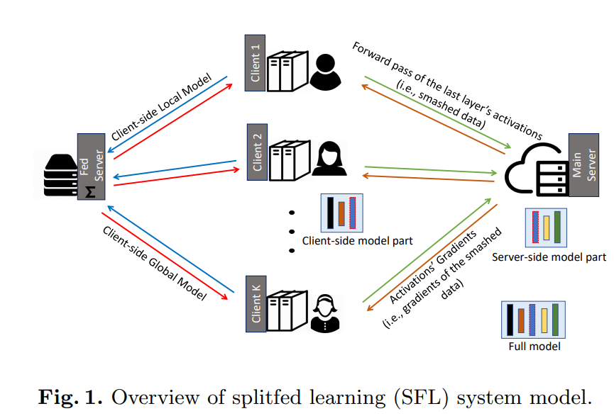Figure 13. Split Federated Learning.

Overview of Split Federated Learning (SFL):

1. Client-side Local Model:
   • Each client (Client 1, Client 2, …, Client K) has a part of the model (Client-side Local Model). This part includes the initial layers of the deep neural network and is run on the client’s local data.
2. Forward Pass:
   • Each client performs a forward pass through its local layers and then sends activations from the final layer, known as smashed data, to the Main Server.
3. Main Server:
   • The main server receives smashed data from the clients and continues processing through the remaining layers of the model (Server-side model part). This part of the model typically includes deeper layers of the neural network, where the most computationally intensive calculations occur.
4. Backpropagation:
   • After completing the forward pass and calculating the loss, the main server performs backpropagation to compute gradients. These gradients, along with the activations (smashed data), are sent back to each client to update the local model.
5. Client-side Global Model:
   • Each client updates its local model based on the gradients received from the server. Once completed, the global model is aggregated and updated on the Fed Server (Federated Server), then sent back to the clients to start a new training cycle.

The SFL model combines the benefits of federated learning and split learning, optimizing computational resource use and ensuring data privacy by not sharing raw data between clients and the main server.

3. Deep Dive into the Paper

Poster of the paper

3.1 Problem

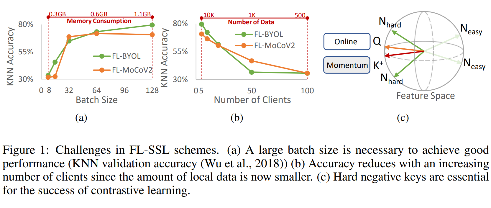Figure 14. Challenges in Unsupervised Federated Learning (FL-SSL).

Figure 1: Challenges in FL-SSL Models

• (a) Large batch size required for good performance: KNN accuracy increases with batch size, but this also raises memory consumption. A large batch size is needed to achieve high performance in KNN validation. The figure shows that as the batch size increases from 8 to 128, KNN accuracy improves for both FL-BYOL and FL-MoCoV2 models, but with a significant increase in memory consumption.

• (b) Accuracy decreases as the number of clients increases: As the number of participating clients grows, each client’s local data becomes smaller, leading to reduced accuracy. Specifically, both FL-BYOL and FL-MoCoV2 models show a drop in KNN accuracy as the number of clients increases from 5 to 100 due to the dispersion and reduction of local data.

• (c) Hard negative keys are crucial for contrastive learning success: In the feature space, using hard negative keys (N_hard) is important for optimizing contrastive learning. Easy negative keys (N_easy) provide less valuable information and do not improve model performance. The figure illustrates that hard negative key samples are critical for enhancing learning in the feature space.

MoCoSFL is an innovative combination of SFL-V1 and MoCo-V2.

• Supports mini-batch training using vector concatenation.
• Utilizes shared feature memory.
• Improves non-IID performance by increasing synchronization frequency.

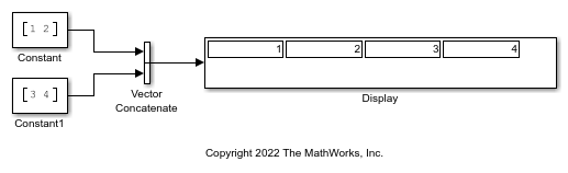Figure 15. Vector concatenation.

3.2 MoCoSFL

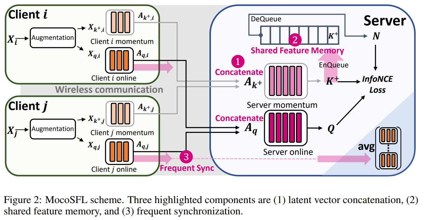Figure 16. MoCoSFL architecture.

The image above shows the architecture of MoCoSFL. In each node, input data X is augmented and passed through the frontend encoder of q and k, then these latent vectors are sent to the server. The server combines all the latent vectors and passes them through the backend encoder k and q to return K+ and Q, then calculates the loss. K+ is placed into shared feature memory. After calculating the loss, backpropagation is used for the backend encoder, which is then sent back to the frontend encoder and frequently synchronized with the federated server using methods like FedAvg to update the global model.

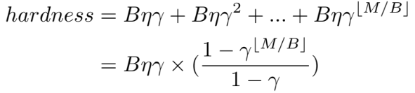Figure 17. Hardness formula.

MoCoSFL alleviates the requirement for large data in self-supervised learning. To evaluate the difficulty of a negative key N in feature memory, we use a similarity measure, which is the dot product between Q and N. The difficulty of a negative key N depends largely on its similarity to the current query key Q, given that N and Q have different true labels.

• B: Batch size
• M: Memory size
• η: Learning rate
• γ: Constant coefficient (γ < 1) for similarity decay of each batch’s negative keys in feature memory due to model updates.

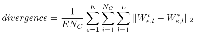Figure 18. Model divergence formula.

Where:

• \(W^*\): Average weights of all nodes
• \(W^i\): Local weights of node \(i\)
• \(L\): Number of layers
• \(E\): Total number of synchronizations
• \(N_C\): Number of clients

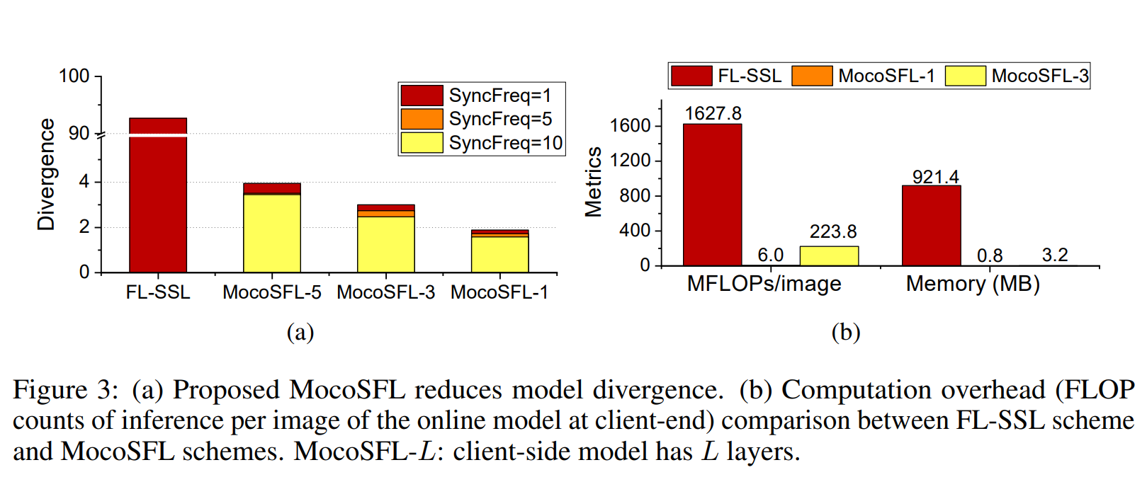Figure 19. MoCoSFL reduces model divergence.

MoCoSFL reduces model divergence compared to FL-SSL methods, as illustrated in chart (a) of Figure 3:

1. Synchronization Frequency (SyncFreq):
   • MoCoSFL uses different synchronization frequencies (1, 5, 10), significantly reducing divergence compared to FL-SSL.
   • As the number of layers on the client-side increases (MocoSFL-5, MocoSFL-3, MocoSFL-1), divergence decreases further.
2. Divergence Level:
   • FL-SSL has the highest divergence (~90), while MocoSFL-1 drops below 5, with higher synchronization frequencies further reducing divergence.
3. Model Divergence Calculation:
   • Model divergence between two models is calculated using the L2 norm of the weight difference.
   • Total divergence in a system among clients can be measured by averaging the weight divergence of local models.

By reducing model divergence, MoCoSFL optimizes the distributed learning process and enhances model accuracy.

3.3 TAResSFL - Target-Aware ResSFL

MoCoSFL has two main issues: high communication cost due to the transmission of latent vectors and vulnerability to Model Inversion Attack (MIA), which threatens client data privacy.

→ TAResSFL, an extension of ResSFL, addresses these issues by: (1) using target-data-aware self-supervised pre-training, and (2) freezing the feature extractor during SFL training. It also employs a bottleneck layer design to reduce communication costs.

In ResSFL, the server performs pretraining against MIA using data from multiple domains. It then sends the pre-trained frontend model to clients for fine-tuning with SFL.

TAResSFL improves pretraining by assuming the server has access to a small portion (<1%) of training data, along with a large dataset from another domain. The pre-trained frontend model provides better transfer learning and remains unchanged during SFL, avoiding costly fine-tuning.

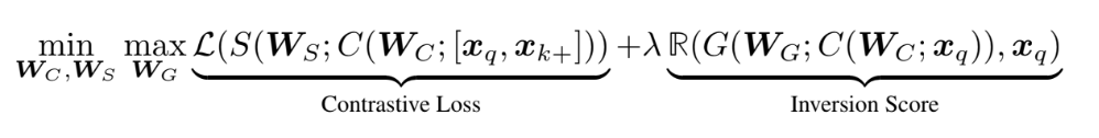Figure 20. TAResSFL loss function formula.

• $W_C$ represents the parameters of the matching feature extractor.
• $W_S$ represents the parameters of the similarity model, used to calculate similarity between the reconstructed and actual inputs.
• $W_G$ represents the parameters of the simulated attack model, responsible for reconstructing activations to a state similar to actual input.
• $x_q$ is the actual input.
• $x_k^+$ is a positive example, often chosen from the same class as $x_q$ to enhance similarity.
• $S$ denotes the similarity function, typically using contrastive loss.
• $R$ represents the regularization term, often incorporating a measure.

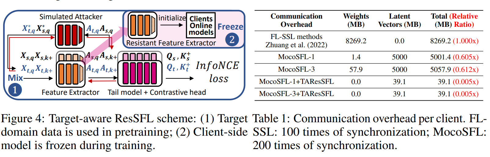Figure 21. TAResSFL scheme.

TAResSFL Scheme:

1. Step 1: Feature Extraction and Simulated Attacker
   • Input data $X_{t,q}^$ and $X_{s,q}^$ are passed through the feature extractor.
   • These features are then processed by the simulated attacker model to reconstruct activations $A_{t,q}$ and $A_{s,q}$.
2. Step 2: Frozen Client-Side Model
   • The client-side models are initialized and then frozen during the training process. This model acts as a resistant feature extractor.
3. Compute InfoNCE Loss
   • Activations from Step 1 are combined with tail models and contrastive heads to compute the InfoNCE loss, optimizing similarity between positive samples and reducing similarity with negative samples.

Main Goal of this scheme is to use target-domain data for pretraining the model, then freeze the client-side model weights during training to minimize communication costs and optimize federated learning.

4. Experiments

Experiment Setup:

• Simulated multiple clients using Linux machines with RTX-3090 GPUs.
• Used datasets CIFAR-10, CIFAR-100, and ImageNet 12. For IID, datasets were randomly and evenly split among clients. For non-IID, randomly assigned 2 classes for CIFAR-10/ImageNet-12 or 20 classes for CIFAR-100 to each client.
• Trained MoCoSFL for 200 epochs with SGD optimizer (initial LR: 0.06).
• Evaluated accuracy using linear probe: trained a linear classifier on the frozen representations. Simplified: model representations (data) → features → linear classifier to evaluate the model’s pre-trained sample extraction capability.

Linear Evaluation: The classifier is trained using the extracted representations as input features, usually with a simple linear layer added to perform classification. This method enables effective transfer learning, as the pre-trained model has learned rich and useful representations from the initial task that can be fine-tuned for the current specific task.

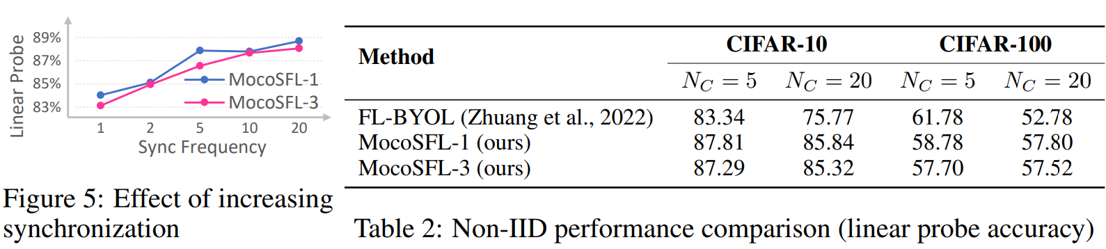Figure 22. Accuracy Performance.

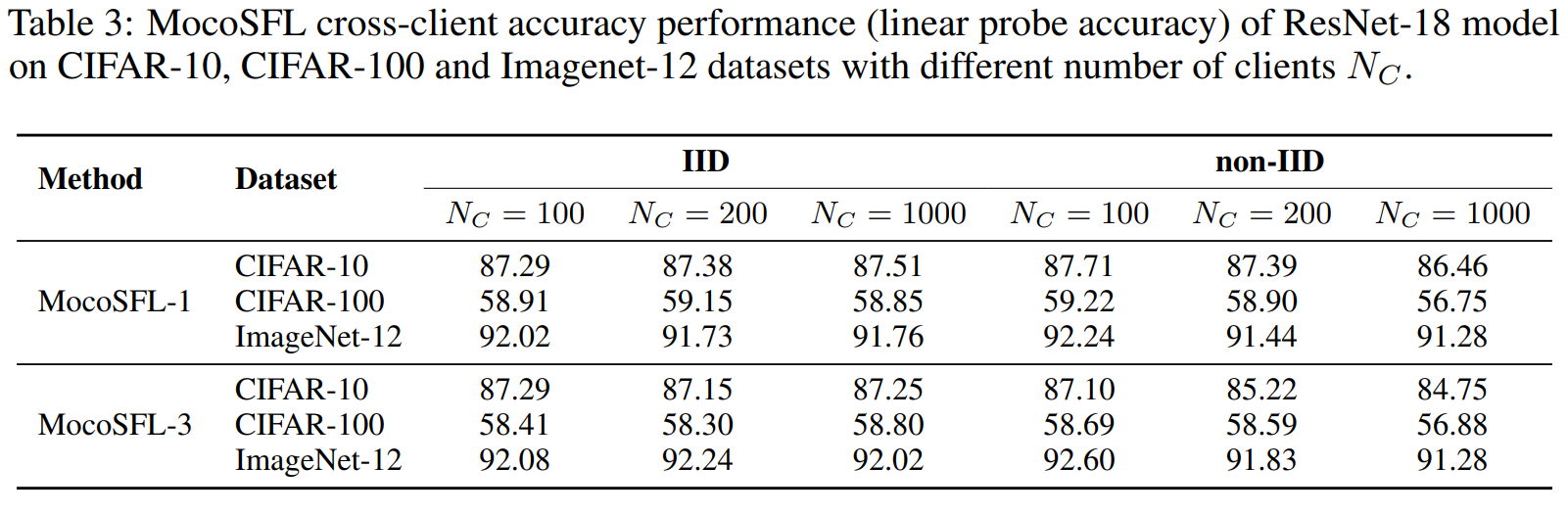Figure 23. Accuracy Performance.

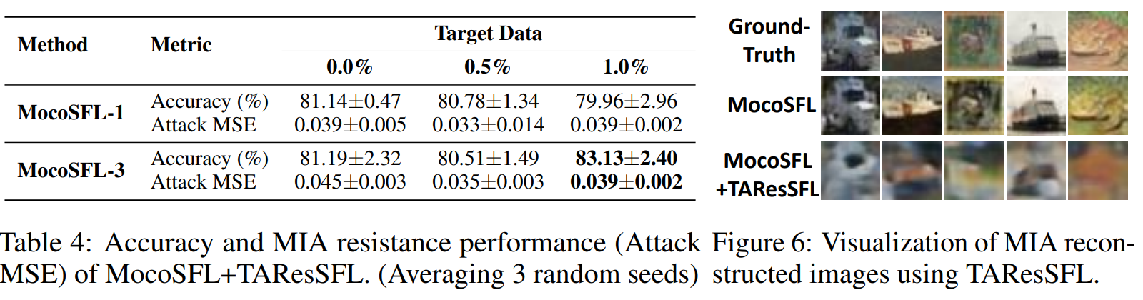Figure 24. Privacy Evaluation.

Comparing hardware resource costs of MoCoSFL, MoCoSFL+TAResSFL (SyncFreq=1/epoch over 200 epochs), and FL-SSL (E=500, SyncFreq=1 every 5 local epochs).

• Raspberry Pi 4B with 1GB RAM served as an actual client, with other clients simulated on PCs.
• MoCoSFL: 1,000 clients, batch size 1, cut layer 3.
• FL-SSL: 5 clients, batch size 128.
• Default data is 2-class non-IID.
• Cost evaluated using ‘fvcore’ for FLOPs and ‘torch.cuda.memory_allocated’ for memory.

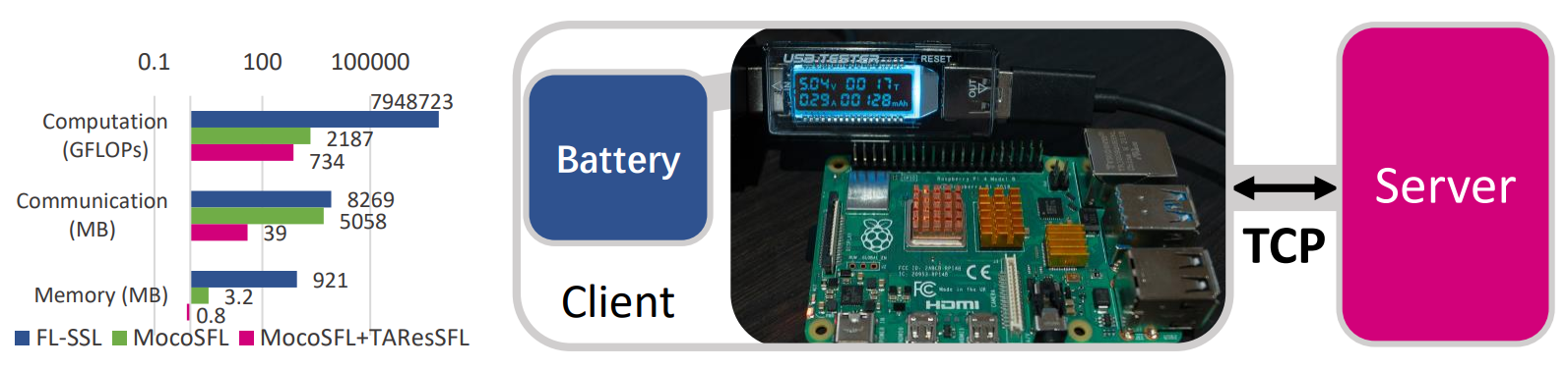Figure 25. Hardware demonstration.

5. References

[1] Momentum Contrast for Unsupervised Visual Representation Learning, Kaiming He et al.

[2] SplitFed: When Federated Learning Meets Split Learning, Chandra Thap et al.

[3] MocoSFL: enabling cross-client collaborative self-supervised learning, Jingtao Li et al.

[4] ResSFL: A Resistance Transfer Framework for Defending Model Inversion Attack in Split Federated Learning, Jingtao Li et al.