

FedPAC: Personalized federated learning with feature alignment and classifier collaboration
Contents
1. Introduction
In this paper, we will explore the FedPAC algorithm, a prominent paper published in the top 5% at the ICLR 2023 conference [1].
The issue with non-IID data in federated learning:
- In federated learning, the data distribution across clients is often not identical (non-IID or heterogeneous).
- Issues with non-IID data: Feature distribution drift, label distribution skew, and concept shift.
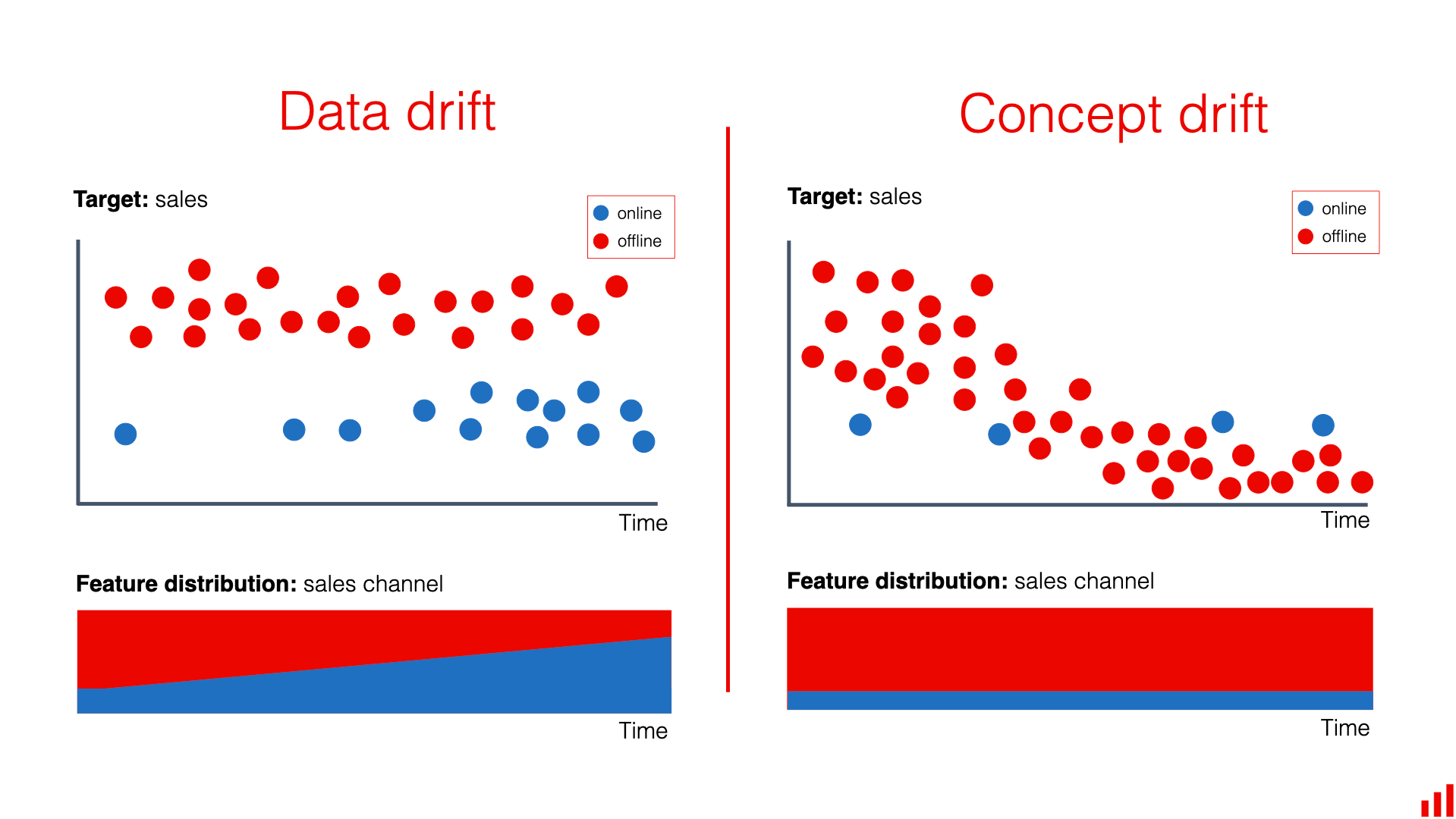 Figure 1. Data drift and Concept drift.
Data drift and Concept drift
Data drift
- Target: Sales
- Description: Data about online and offline sales changes over time. The distribution of features (sales channel) also shifts, with offline sales increasing and online sales decreasing over time.
- Outcome: The model may not perform well due to changes in the input data distribution.
Concept drift
- Target: Sales
- Description: Online and offline sales both gradually decline over time. However, the distribution of features (sales channel) does not change significantly.
- Outcome: The model needs to be updated to reflect changes in the relationship between features and the target.
Many studies focus on optimizing local learning algorithms by leveraging well-designed target adjustment techniques. Examples include:
- FedProx (Li et al., 2020b): Adds a proximal term to the local training objective to keep the updated parameters close to the downloaded global model.
- SCAFFOLD (Karimireddy et al., 2020b): Introduces control variates to adjust for drift in local updates.
- MOON (Li et al., 2021b): Uses adversarial loss to improve representation learning.
Why Personalized Federated Learning?
- Non-IID data makes it challenging to build a single global model applicable to all clients.
- Personalized federated learning has been developed to learn a customized model for each client, improving performance on local data while still benefiting from collaborative learning.
Common methods for Personalized Federated Learning (Personalized FL) include:
Additive model mixture: Performs a linear combination of local and global models.
Examples: L2CD, APFL.Multi-task learning with model dissimilarity penalization.
Examples: FedMTL, pFedMe, Ditto.Parameter decoupling of feature extractor and classifier.
Examples: FedPer, LG-FedAVG, FedRep.Clustered FL: Groups similar clients and learns multiple global models within clusters.
Examples: FedFoMo, Fed AMP.
Other federated learning (FL) methods for specific clients include:
- FedGP: Based on Gaussian processes.
- pFedHN: Activated by hypernetwork on the server side.
- FedEM: Learns a mixture of multiple global models.
- Fed-RoD: Uses balanced softmax to learn a common model and original softmax for personalized outputs.
- FedBABU: Keeps the global classifier fixed during feature representation learning and performs local adjustments through fine-tuning.
- kNN-Per: Applies a combination of the global model and local kNN classifiers for better personalization.
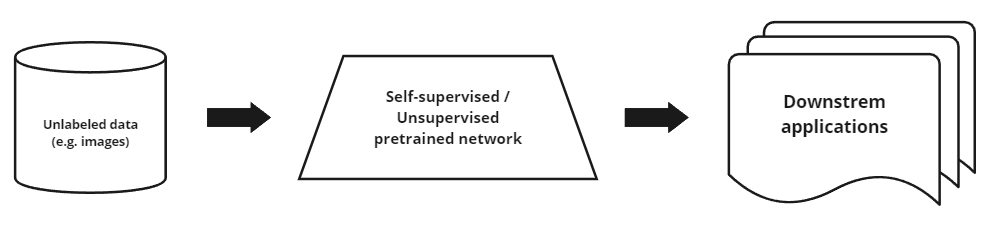 Figure 2. Application of unsupervised learning.
Representation Learning and Downstream Application
- Representation Learning: Automatically learns useful features from raw data.
- Downstream Application: Uses the learned representations from representation learning to solve practical tasks or problems.
Multi-Tasks Learning
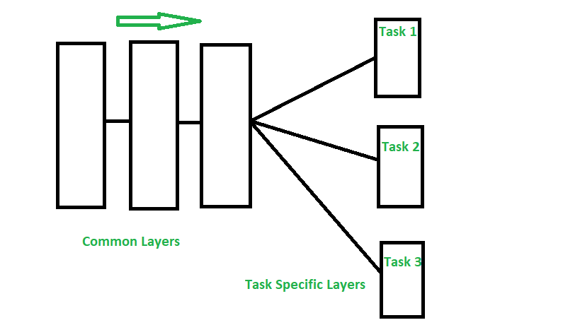 Figure 3. Multi-Tasks Learning.
The image above illustrates the deep learning architecture for multi-task learning.
Common Layers: These layers are shared across different tasks. They are responsible for extracting common features from the input data.
Task Specific Layers: These layers are specialized for each specific task. After passing through the common layers, the output is divided into separate branches, each corresponding to a specific task such as Task 1, Task 2, and Task 3.
This architecture allows the model to leverage information from different tasks, improving overall performance by learning common features while still ensuring task-specific specialization.
Main contributions of the paper:
- Primarily considers the label distribution shift and classification task scenarios.
- Studies federated learning from the perspective of multi-task learning by leveraging both shared representation and inter-client classifier.
2. Proposed framework
Problem setup
Consider:
- There are $m$ clients and one central server.
- $X$ is the input space, $Y$ is the label space, and $K$ is the number of categories.
- Each client $i$ has its own data $P^{(i)}_{XY}$ and it is assumed that $P^{(i)} \neq P^{(j)}$.
- The loss function $\ell : X \times Y \rightarrow \mathbb{R}^+$ is provided by the local model $w_i$.
- $W = (w_1, w_2, \ldots, w_m)$.
The optimization objective is represented as follows:
\[\min_{\mathbf{W}} \left\{ F(\mathbf{W}) := \frac{1}{m} \sum_{i=1}^{m} \mathbb{E}_{(x, y) \sim P^{(i)}_{XY}} \left[ \ell(w_i; x, y) \right] \right\}\]- The true underlying distribution is not accessible. The goal is achieved through empirical risk minimization (ERM).
- Assume each client has access to $n_i$ IID data points sampled from $P^{(i)}_{XY}$, denoted by \(D_i = \{(x^{(i)}_l, y^{(i)}_l)\}_{l=1}^{n_i}, \hat{P}^{(i)}_{XY}\) Assume \(\hat{P}^{(i)}_{Y} = P^{(i)}_{Y}\)
Sharing feature representation
The feature embedding function $f: \mathcal{X} \rightarrow \mathbb{R}^d$ is a learned network parameterized by $\Theta_f$ and $d$ is the dimension of $z$, with $z = f(x)$ and $\hat{y} = g(z)$.
$g(z)$ is parameterized by $\Phi_g$, and the entire model parameters are $\mathbf{w} = {f, \Phi}$.
Sharing feature layers can reduce the data scarcity issue of clients, which causes overfitting, but local updates increase overfitting and parameter diversity.
→ A new regularization term is proposed to address this issue.
Clients update their local models with a new regularization term that incorporates global feature centroids to improve generalization.
- $f_{\phi_i}(x_j)$ is the local feature embedding of data point $x_j$.
- $c_{y_j}$ is the global feature centroid corresponding to class $y_j$.
- $\lambda$ is a hyperparameter to balance between supervised loss and regularization loss.
Classifier collaboration
- Enhance performance by aggregating classifiers from similar clients, reducing variance and improving local models through knowledge transfer between clients.
- To evaluate the similarity and transferability between clients, we perform a linear combination of received classifiers for each client $ i $ to minimize local test loss:
- Each coefficient $ \alpha_{ij} \geq 0 $ is determined by minimizing the expected local test loss through an optimization problem:
- To enhance collaboration, the coefficients $ \alpha_i $ need to be adaptively updated during training.
3. Algorithm design
Local training procedure
In each local training round $t$, the model is updated with the global aggregation received for the feature layers and adjusts the corresponding private classifiers, then applies stochastic gradient descent to train both parts of the model parameters.
- Step 1: Fix $\theta_i$, Update $\phi_i$. Train $\phi_i$ on private data using gradient descent for one epoch:
where $\xi_i$ denotes the mini-batch of data, and $\eta_g$ is the learning rate for updating the classifier.
- Step 2: Fix the new $\phi_i$, Update $\theta_i$. After obtaining the new local classifier, continue training the local feature extractor based on both private data and global feature centroids for several epochs:
where $\eta_f$ is the learning rate for updating the feature layers, $c^{(t)} \in \mathbb{R}^{K \times d}$ is the set of global feature centroid vectors for each class, and \(K = |\mathcal{Y}|\) is the total number of classes.
Before updating the local feature extractor, each client extracts the local feature statistics $\mu_i^{(t)}$ and $V_i^{(t)}$ to estimate the combined weights of the classifier. After updating the feature extractor, the local feature centroids for each class are calculated.
\[\hat{c}_{i,k}^{(t+1)} = \frac{\sum_{l=1}^{n_i} \mathbb{1}(y_l^{(i)} = k) f_{\theta_i^{(t+1)}}(x_l^{(i)})}{\sum_{l=1}^{n_i} \mathbb{1}(y_l^{(i)} = k)}, \forall k \in [K].\]Global aggregation
Global feature representation. Similar to popular algorithms, the server performs a weighted average of local feature layers with each weight determined by the local data size.
\[\tilde{\theta}^{(t+1)} = \sum_{i=1}^{m} \beta_i \theta_i^{(t)}, \quad \beta_i = \frac{n_i}{\sum_{i=1}^{m} n_i}.\]Classifier aggregation. The server uses the received feature statistics to update the combined weight vector $\alpha_i$ by solving (11) and performs classifier aggregation for each client $i$.
Update global feature centroids. After receiving the local feature centroids, the following centroid aggregation operation is performed to create an estimated global centroid $c_k$ for each class $k$.
\[c_k^{(t+1)} = \frac{1}{\sum_{i=1}^{m} n_{i,k}} \sum_{i=1}^{m} n_{i,k} \hat{c}_{i,k}^{(t+1)}, \quad \forall k \in [K].\]4. Experiments
Experiments setup
Datasets: EMNIST, Fashion-MNIST, CIFAR-10, and CINIC-10.
- Data Partitioning:
- Clients have uniform data sizes, with 20% sampled uniformly and the rest from dominant classes.
- Clients are grouped by shared dominant classes, with small local training data.
- Testing data matches training data.
Compared Methods: Baselines include Local-only, FedAvg, FedAvgFT, APFL, pFedMe, Ditto, LG-FedAvg, FedPer, FedRep, FedBABU, Fed-RoD, kNN-Per, FedFomo, and pFedHN.
- Training Settings:
- Mini-batch SGD is used as a local optimizer for all approaches, with 5 local training epochs.
- 200 global communication rounds are set for all datasets.
Results
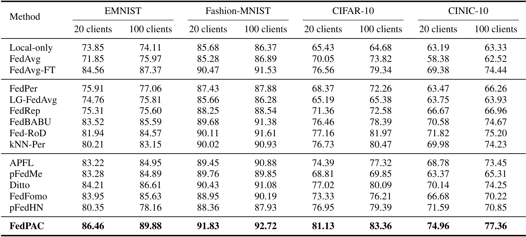 Figure 4. Comparison of test accuracy (%) across different datasets.
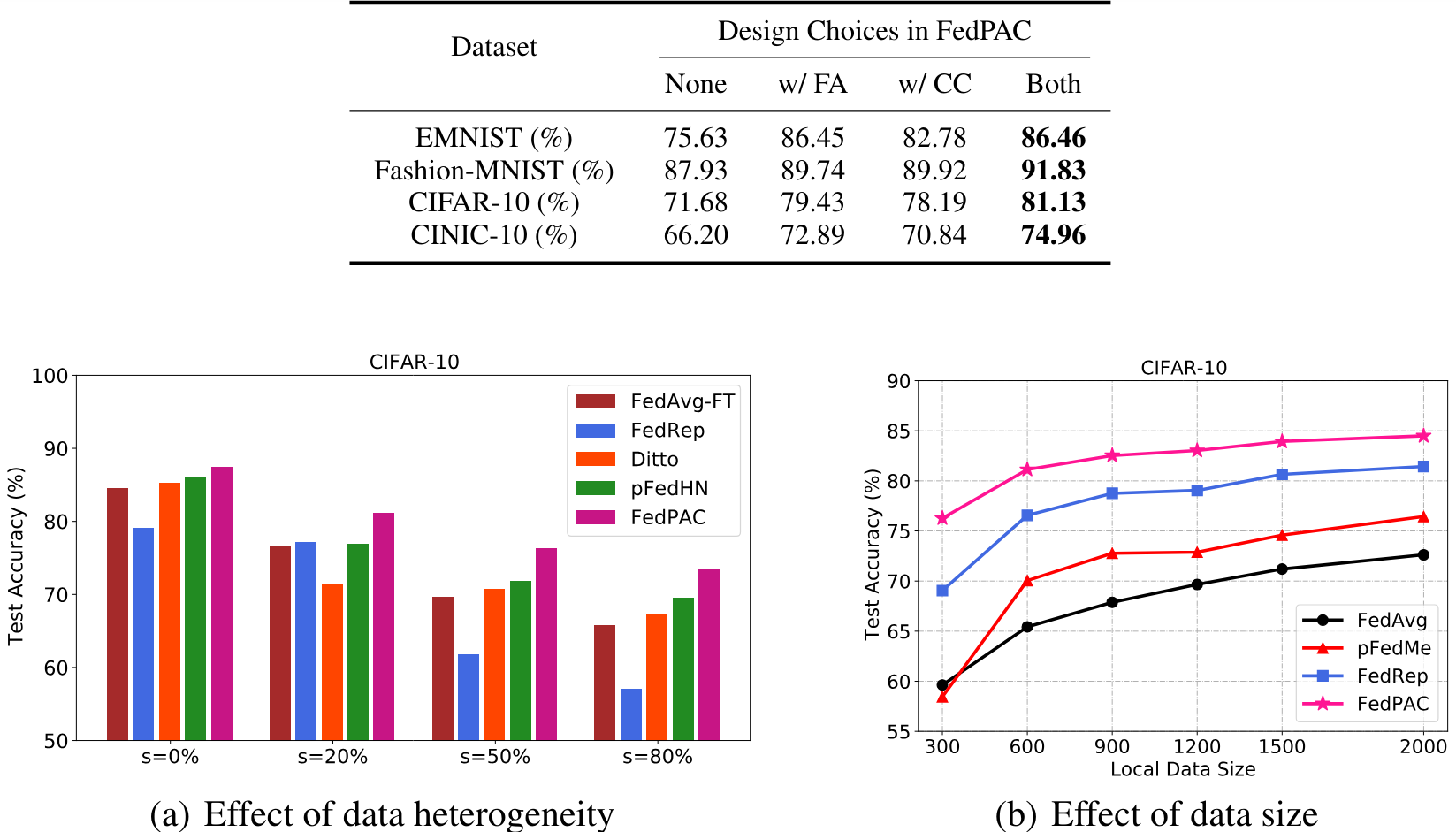 Figure 5. Performance comparison on the CIFAR-10 dataset with varying data heterogeneity and local data size.
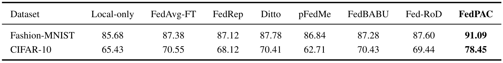 Figure 6. Test accuracy (%) under concept shift.
5. References
[1] Personalized Federated Learning with Feature Alignment and Classifier Collaboration, Jian Xu et al.