Federated Learning: An Overview

Posted Aug 15, 2024

By Anh Dinh 9 min read

1. Introduction
2. Key Features of Federated Learning
3. Types of Federated Learning Based on Data Distribution Characteristics
4. Federated Learning Algorithms
5. Variants of Federated Learning
6. References

1. Introduction

Currently, training AI models with traditional machine learning methods faces two main challenges. First, data is often isolated and distributed across many locations in most industries. Second, there are increasing data privacy policies. To address these issues, a new distributed machine learning method has been proposed by Google’s engineers [1].

Federated Learning, also known as collaborative learning, is a technique in machine learning that enables training AI models on data across devices, servers, and distributed data centers without centralizing the data, yet still achieving performance comparable to traditional machine learning methods [1][2].

2. Key Features of Federated Learning

2.1 Iterative Learning

To ensure the final global model performs well, Federated Learning relies on an iterative process divided into interactions between Nodes and Servers, called federated learning rounds. Each round includes sending the global model to participating Nodes for local training with local data, then aggregating these local models to create a new global model [3].

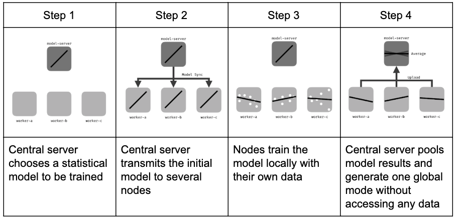Figure 1. Key processes of Federated Learning.

The iterative federated learning process includes the following main steps [4]:

Initialization: Based on a small dataset at the Server, an initial machine learning model is selected and trained.
Node Selection: A subset of Nodes is chosen to participate in training. Nodes not selected will wait for future rounds.
Configuration: The Server sends hyperparameters to the Nodes for local training (mini_batch, local_iteration, etc.).
Feedback: After training, Nodes send their local models back to the Server for aggregation. If any selected Node fails to respond (e.g., due to connection issues), it will be asked to send feedback in later rounds.
Completion: Once the desired results are achieved (number of global rounds or specific performance threshold), the Server finalizes the global model and ends the process.

2.2 Non-IID Data

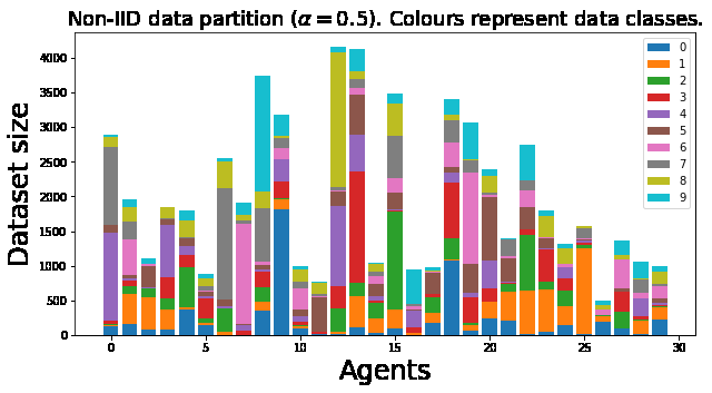Figure 2. Example of non-IID data.

Typically, data distributed across Nodes is non-IID (non-independent and identically distributed). Non-IID data is described based on probabilistic analysis of the relationship between features and labels at each Node. This allows each Node’s contribution to be separated based on the specific distribution available locally. Non-IID data has the following key characteristics [3]:

Covariate Shift: Local Nodes may store examples with different statistical distributions compared to other Nodes. For instance, handwriting styles may vary between people.
Prior Probability Shift: Local Nodes may store different labels. This can occur if datasets are divided by region or location, such as different animal images in various countries.
Concept Drift: Local Nodes may have the same labels but different features.
Concept Shift: Local Nodes may have the same features but different labels.
Unbalancedness: The amount of data available at each local Node can vary in size.

2.3 Security

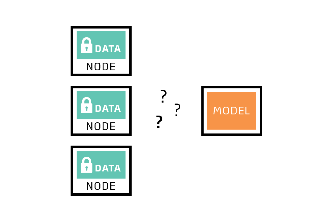Figure 3. Data Privacy.

Security is a top priority in federated learning. With increasing attention to data privacy, many policies have been implemented [5]. The main goal of federated learning is to enable machine learning to realize its potential while ensuring data safety.

The key idea of federated learning is to train models with local data and only exchange model parameter updates. This helps to protect data fully at the local Node, preventing data leakage while participating in collective learning with other Nodes [1].

3. Types of Federated Learning Based on Data Distribution Characteristics

In federated learning, data often has diverse distributions and characteristics. To fit different tasks, there are types of federated learning based on data partitioning and characteristics [1].

Notation:

\(i\) is the i-th node in \(\{1, \ldots, N\}\) nodes
\(D_i\) denotes the data matrix at node \(i\)
\(X_i\) is the feature space of node \(i\)
\(Y_i\) is the label space of node \(i\)
\(I\) denotes the ID space
A dataset at a node looks like \((I, X, Y)\)

3.1 Vertical Federated Learning

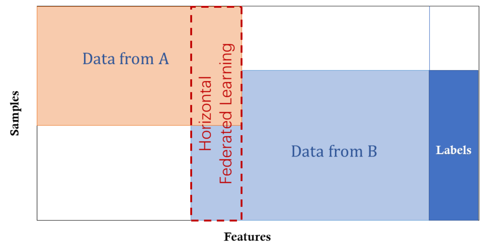Figure 4. Vertical Federated Learning.

Vertical Federated Learning, also known as feature-based federated learning, applies when two datasets have the same ID space but different feature spaces. For example, consider two different companies in the same city: a bank and an e-commerce platform. They likely have many overlapping customers, but the bank records spending behavior and credit ratings, while the e-commerce platform tracks search and purchase history, resulting in very different features. Suppose we want both to have a model predicting purchases based on customer and product information [1].

Vertical Federated Learning involves combining different features and training a model privately based on loss and gradients between two cooperating parties. In this system, identities and statuses of participants are the same, and the federated system helps establish a common model. In this system, we have the following characteristics [1]:

\[X_i \neq X_j, \quad Y_i \neq Y_j, \quad I_i = I_j, \quad \forall D_i, D_j, \, i \neq j\]

3.2 Horizontal Federated Learning

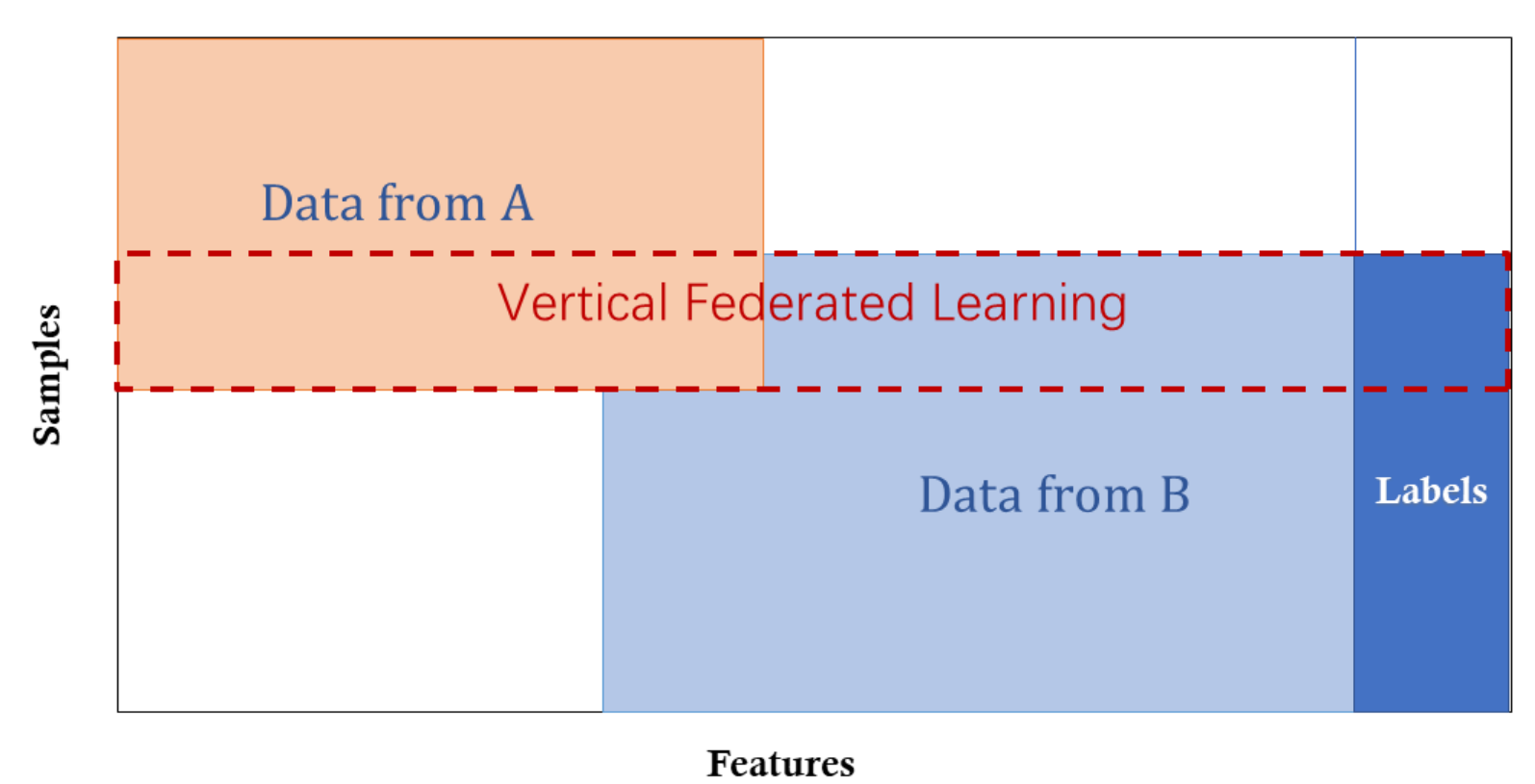Figure 5. Horizontal Federated Learning.

Horizontal Federated Learning, also known as sample-based federated learning, occurs when feature spaces are the same, and different parties contribute additional samples to enrich the data. For example, two regional banks with different customer groups but similar business activities would use horizontal federated learning. An example is Google’s 2017 proposal for horizontal federated learning as a solution to update model parameters for Android phones. In this approach, an Android user updates their local model parameters and uploads them to the Android cloud, training a centralized federated model with other Android devices. In this system, we have the following characteristics [1]:

\[X_i = X_j, \quad Y_i = Y_j, \quad I_i \neq I_j, \quad \forall D_i, D_j, \, i \neq j\]

3.3 Transfer Federated Learning

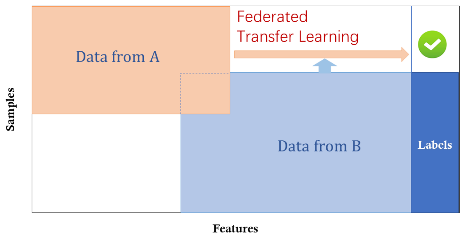Figure 6. Transfer Federated Learning.

Transfer Federated Learning is more special. It uses federated learning methods to train models for domains that have small datasets or low data quality. Transfer federated learning assumes that only a limited amount of data is available for model training and the data quality is not high enough to train a high-performance model [6].

In transfer federated learning, local nodes use a pre-trained global model as a starting point. This approach involves transferring knowledge from one domain to another, improving learning performance with limited data [7]. This is especially useful for small sample learning tasks [6].

In this system, we have the following characteristics [6]:

\[X_i \neq X_j, \quad Y_i \neq Y_j, \quad I_i \neq I_j, \quad \forall D_i, D_j, \, i \neq j\]

4. Federated Learning Algorithms

Several algorithms have been developed to enhance the performance and efficiency of federated learning systems:

Federated Stochastic Gradient Descent (FedSGD): FedSGD is a basic federated learning algorithm where local models are trained using stochastic gradient descent and then aggregated to update the global model [8].
Federated Averaging (FedAvg): FedAvg combines local training using stochastic gradient descent with model averaging to improve performance and efficiency [8].
Federated Proximal (FedProx): FedProx introduces a proximal term to the objective function to handle heterogeneity among local models, improving convergence and robustness [8].

5. Variants of Federated Learning

5.1 FedSGD

The basic optimization algorithm for Federated Learning is built on Stochastic Gradient Descent (SGD). Federated Learning with Stochastic Gradient Descent (FedSGD) computes gradients for each batch (where each batch represents each Node) during a Federated Learning round [6].

Common settings when implementing model training with FedSGD are a ratio of \(C = 1\), \(B = \infty\), \(E = 1\), and a fixed \(\eta\). Nodes compute \(g_k = \nabla F_k(w_t)\) and send \(g_k\) back to the Server. The Server then aggregates the new global model using the following formula [6]:

\[w_{t+1} \leftarrow \nabla f(w_t) \quad \text{where} \quad \nabla f(w_t) = w_t - \eta \sum_{k=1}^{K} \frac{n_k}{n} g_k \quad (3)\]

This approach seems effective but requires a large number of rounds to train a good model [7].

5.2 FedAvg

The SGD-based approach (3) can also be implemented as follows: Nodes compute \(g_k\) and update the local model as \(w_{t+1}^k \leftarrow w_t - \eta g_k\), then send \(w_{t+1}^k\) back to the Server. The Server then aggregates the new global model using the formula:

\[w_{t+1}^k \leftarrow w_t - \sum_{k=1}^{K} \frac{n_k}{n} g_k \quad (4)\]

This implementation averages local models, so it is called Federated Averaging (FedAvg) [6].

The FedAvg implementation uses three main parameters: the ratio of Nodes selected per Federated Learning round (\(C\)), the number of local epochs (\(E\)), and the local batch size (\(B\)). Setting \(C = 1\), \(B = \infty\), \(E = 1\) corresponds to SGD. For each Node with \(n_k\) data, the number of updates per round is \(u_k = \frac{E \cdot n_k}{B}\) [6].

5.3 FedProx

With the FedAvg algorithm, each Federated Learning round selects a fraction \(C\) (0 < \(C\) < 1) of Nodes to participate in the learning process. These Nodes optimize the local model using Gradient Descent, with a fixed parameter \(E\) (local epoch), so the local model is trained \(E\) times [6]. Since data across Nodes is not identical, some Nodes may converge earlier while others may not. Often, local models converge early and diverge from the convergence point of the global model [8]. To minimize this issue, a penalty parameter \(\mu\) is used to control the discrepancy between \(w_t\) and \(w_{t+1}^k\). The penalty term is added to the local loss function as follows [8]:

\[h(w; w_0) = F(w) + \frac{\mu}{2} \|w - w_0\|^2 \quad (5)\]